Debunking Convolutional Neural Networks (CNN) with practical examples

Hello and welcome to the second post on Debunking Neural Network series In the previous post, we saw what is Deep Learning and how it is radically transforming industries. Next, we had a look at Artificial Neural Networks which are the driving forces behind the immense potential of DL. Then we also had a brief look at Google’s Deep Learning framework called Tensorflow. To make things a little bit easy we utilized Keras’ powerful interface for Tensorflow to construct our programs. Finally, we had a look at how Artificial Neural Networks & DL can be used to solve seemingly difficult problems such as predicting housing prices, classifying mail as a Spam/not spam.

All those examples we saw in the last post were, in some or the other form of text and numbers. But have you ever wondered how would these Neural Networks perform if the data is in the form of Images or Videos? This post will be about that special type of Neural Network called Convolutional Neural Networks which are the go-to architecture when working with images.

Originally the Convolutional Neural Network architecture was introduced by Yann LeCun back in 1998. It took almost one and a half-decade to get big attention to convolutional networks when, in 2012, the ImageNet competition was won by a team using this architecture.

A Primer on CNN’s:

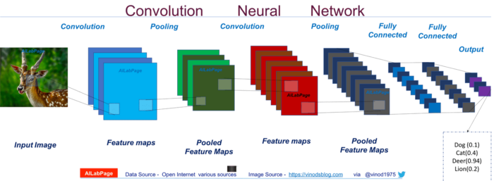
There are four main operations in the ConvNet shown above:

1. Convolution
2. Non Linearity (ReLU)
3. Pooling
4. Classification (Fully Connected Layer)

STEP-1: Convolution Operation

Every image can be represented as a matrix of pixel values. The primary purpose of Convolution in the case of a ConvNet is to extract features from the input image. Convolution preserves the spatial relationship between pixels by learning image features using small squares of input data. Convolution operation can be understood using the animation.

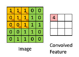
In CNN terminology, the 3×3 matrix is called a ‘filter‘/‘kernel’/‘feature detector’ and the matrix formed by sliding the filter over the image and computing the dot product is called the ‘Convolved Feature’/‘Activation Map’/‘Feature Map‘.

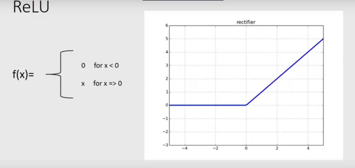
STEP-2: Non-Linearity

ReLU stands for the Rectified Linear Unit and it is a Non-Linear Mathematical operation. ReLU is an element-wise operation (applied per pixel) and replaces all negative pixel values in the feature map by zero. The purpose of ReLU is to introduce non-linearity in our ConvNet since the Convolution operation itself is a linear operation, so we account for non-linearity by introducing a non-linear function.

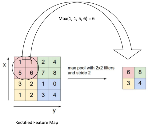
STEP-3: Pooling

Pooling is a form of dimensionality reduction technique. Pooling reduces the dimensionality of each feature map while retaining the crucial information. Pooling can be of different types: Max, Average, Sum, etc. Below shows an example of Max Pooling operation on a Rectified Feature map (obtained after convolution + ReLU operation) by using a 2×2 window.

STEP-4: Classification

The Fully Connected layer is nothing but a simple Multi-Layer Perceptron that uses a softmax activation function in the output layer. The purpose of this Fully Connected layer is to use high-level features, abstracted from previous layers, to classify the input image into various classes based on the training dataset. Traditional Machine Learning classifiers (SVM, Logistic regression) can also be used.

The above explanation is a very brief overview of the terminologies used in CNN’s understanding. I would highly encourage you to look at the reference section of this post and go through all the mentioned articles thoroughly to get a strong understanding of all the underlying principles of CNN before starting to code.

Now that we have a theoretical understanding of what CNN’s are, we can start to make our very own models that will try to solve classification problems for us.

It is always a good practice to create a new Virtual Environment every time you start a new project in your system. This way you can ensure that your libraries from one Environment will not mess up with the libraries from another Environment. Or better yet it won’t even mess with your system-wide installations.

In my previous post, I have described the steps to create a Virtual Environment in your system and also to install all the necessary libraries. In short, steps to create your Deep Learning environment.

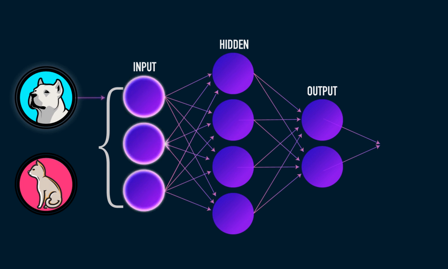
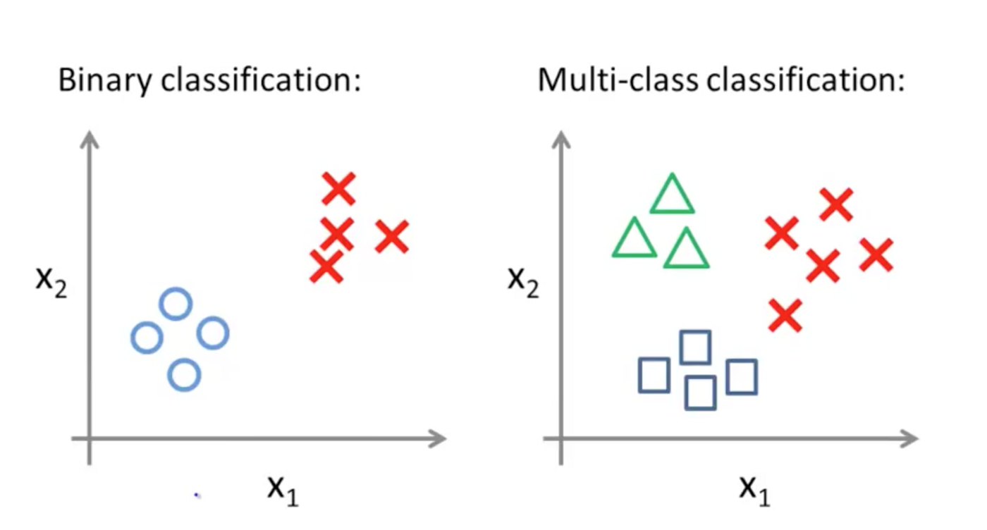
This part will be divided into two parts. The first part will be classifying the input image into one of the two categories i.e Binary Classification. The second part will be to classify the input image into one of the 100 categories i.e Multi-Class Classification.

Part-1: Binary Classification of images

Below shows the code that tries to Classify input images into either a cat or a dog using Dense Convolutional Neural Network with Tensorflow and Keras. You can download the dataset for this problem from HERE.

Tearing the code:

If you have followed my post on Artificial Neural Network you already know this part. We import all the libraries and modules which are essential for creating the model.

from keras.models import Sequential
from keras.layers import Conv2D, MaxPooling2D, Flatten, Dense, Dropout
from keras.preprocessing.image import ImageDataGenerator
from keras.callbacks import EarlyStopping
import matplotlib.pyplot as plt



After importing the modules we initiate a Sequential model instance from Keras and add Convolutional layers, Pooling layers, and the FC layers. On line 22 we add our first Convolutional Layer with the following parameters:

1. Number of nodes — 32
2. Filter size — 3x3
3. The shape of the input images — 64x64x3 i.e. Rows x Column x Channels
4. Activation function- Rectified Linear Unit(ReLU)

On line 23 we add in our Pooling layer with a matrix size of 2x2.

On line 53 we add another layer that flattens the Convolutional layer to 1D. This step is important to do because The output of all the Convolutional layer and Pooling layer is in multiple channels that cannot be directly fed to the Dense FC network. Finally, we add our fully connected layer of 128 nodes. The last layer is the classifier itself with a Sigmoid activation function with the number of nodes equalling to the number of classes.

classifier = Sequential()

classifier.add(Conv2D(32,(3, 3), input_shape=(64, 64, 3),activation='relu'))
classifier.add(MaxPooling2D(pool_size = (2, 2)))
classifier.add(Dropout(0.25))

classifier.add(Conv2D(32, (3, 3), activation = 'relu'))
classifier.add(MaxPooling2D(pool_size = (2, 2)))
classifier.add(Dropout(0.25))

classifier.add(Conv2D(64, (3, 3), activation = 'relu'))
classifier.add(MaxPooling2D(pool_size = (2, 2)))
classifier.add(Dropout(0.25))

classifier.add(Conv2D(128, (3, 3), activation = 'relu'))
classifier.add(MaxPooling2D(pool_size = (2, 2)))
classifier.add(Dropout(0.25))

classifier.add(Flatten())

classifier.add(Dense(units = 128, activation = 'relu')) classifier.add(Dropout(0.25))
classifier.add(Dense(units = 1, activation = 'sigmoid'))



In the next lines, we compile the created model with a few parameters like losses, optimizers, etc.

classifier.compile(
    optimizer = 'adam',
    loss = 'binary_crossentropy',
    metrics = ['accuracy']
    )


Next up we create an “ImageDataGenerator” instance from Keras that will randomly zoom, rescale, flip(horizontally & vertically) the images. This step is called DATA AUGMENTATION. Data Augmentation helps in creating a model that is robust and variance tolerant. This means that the model will still be able to perform well even if the input image is distorted in some manner(zoomed, sheared, blurred, flipped, etc). After creating this instance, we pass in our training data to it in batches.

train_datagen = ImageDataGenerator(
    rescale=1./255,
    shear_range=0.2,
    zoom_range=0.2,
    horizontal_flip=True,
    vertical_flip = True
    )

training_set = train_datagen.flow_from_directory(
    '../dataset/training_set',
    target_size=(64, 64),
    batch_size=32,
    class_mode='binary'
    )


Performing a similar step of data augmentation for the testing dataset we only rescale it.

test_datagen = ImageDataGenerator(rescale=1./255)

test_set = test_datagen.flow_from_directory(
    '../dataset/test_set',
    target_size=(64, 64),
    batch_size=32,
    class_mode='binary'
    )


We then pass in our augmented data to the fit_generator method instead of the fit method. This is done due to the output format of the ImageDataGenerator method.

Notice we have declared a parameter called stopper which calls ‘Early stopping’.Early Stopping is an amazing utility in Keras wherein you pass a Validation Patience and a loss monitor. What this does is it monitors the model’s performance based on its validation loss(‘val_loss’) and if the performance does not change after 20 epochs(‘Validation Patience’), the training of the model will stop. Thus taking care of our time while training the model. We then fit the model with the training dataset.

VALIDATION_PATIENCE = 3
stopper = EarlyStopping(monitor='val_loss', patience=VALIDATION_PATIENCE)

classifier.fit_generator(
    training_set,
    steps_per_epoch=8000,
    callbacks = [stopper],
    epochs=25,
    validation_data=test_set,
    validation_steps=2000,
    use_multiprocessing = True
    )



Part-2: Multi-Class Classification(Cifar 100)

Below shows the code that tries to Classify input images into one of the 100 mentioned classes using Dense Convolutional Neural Network with Tensorflow and Keras(Duh…). Keras comes shipped with the CIFAR100 dataset off the shelf. For the first time you run the code it will download the dataset and store it locally. Also, if it suits you, you can download the CIFAR100 dataset and perform your data preprocessing on it.

Tearing the code:

The first and foremost part in almost every Python program is importing all the necessary libraries.

from keras .models import Sequential
from keras.layers import Conv2D, MaxPooling2D, Flatten, Dense, Dropout
from keras.utils import np_utils
from keras.callbacks import EarlyStopping
import matplotlib.pyplot as plt


Next, we load in our dataset. since we are using TensorFlow as backend, we need to reshape the feature matrix as being: 1) The number of samples, 2)Number of rows, 3)Number of columns, 4) Number of channels. After reshaping it we normalize the inputs.

from keras.datasets import cifar100

(X_train, y_train), (X_test, y_test) = cifar100.load_data(label_mode='fine')

X_train = X_train.reshape(X_train.shape[0], 32, 32, 3)
X_test = X_test.reshape(X_test.shape[0], 32, 32, 3)

X_train = X_train.astype('float32')/255
X_test = X_test.astype('float32')/255

y_train = np_utils.to_categorical(y_train, 100)
y_test = np_utils.to_categorical(y_test, 100)



Then comes the FUN part. To create a model we need to Initiate the Sequential model from Keras and add in the Convolutional, Pooling, and Dense FC layers. The last FC layer will have 100 nodes corresponding to the number of classes in the dataset.

classifier = Sequential()

classifier.add(Conv2D(64, (3, 3), activation = 'relu', input_shape = (32, 32, 3)))
classifier.add(MaxPooling2D(pool_size = (2, 2)))
classifier.add(Dropout(0.25))

classifier.add(Conv2D(64, (3, 3), activation = 'relu'))
classifier.add(MaxPooling2D(pool_size = (2, 2)))
classifier.add(Dropout(0.25))

classifier.add(Conv2D(128, (3, 3), activation = 'relu'))
classifier.add(MaxPooling2D(pool_size = (2, 2)))
classifier.add(Dropout(0.25))

classifier.add(Flatten())

classifier.add(Dense(units = 128, activation = 'relu'))
classifier.add(Dropout(0.25))

classifier.add(Dense(units = 128, activation = 'relu'))
classifier.add(Dropout(0.25))

classifier.add(Dense(units = 128, activation = 'relu'))
classifier.add(Dropout(0.25))

classifier.add(Dense(units = 100, activation = 'softmax'))



We define a few parameters to pass into the compile and fit method.

epochs = 10000
batch_size = 256
VALIDATION_PATIENCE = 20
classifier.compile(optimizer = 'rmsprop', loss = 'categorical_crossentropy', metrics = ['accuracy'])

stopper = EarlyStopping(monitor='val_loss', patience=VALIDATION_PATIENCE)

classifier.fit(X_train, y_train, batch_size=100, callbacks=[stopper], validation_data = (X_test, y_test), epochs=epochs, shuffle = True)



That will be it for the fun part of the post. You have earned yourself a big cup of coffee by completing this

Summary of what we did:

1. A very brief history of CNN and its inception.
2. Theoretical understanding of the core underlying principles of CNN.
3. How to use CNN for Binary Classification and Multi-class Classification.

REFERENCES:

1. https://adeshpande3.github.io/adeshpande3.github.io/A-Beginner's-Guide-To-Understanding-Convolutional-Neural-Networks-Part-2/
2. http://www.wildml.com/2015/11/understanding-convolutional-neural-networks-for-nlp/
3. https://www.codeproject.com/Articles/1264962/ANNT-Convolutional-neural-networks
4. https://ujjwalkarn.me/2016/08/11/intuitive-explanation-convnets/

You can find a well commented and structured code along with reference notes on my Github.

Also, make sure to check out my first post on Artificial Neural Networks in this Debunking Neural Network series.

Ciao Adios ! Until next time. !!!